Source and Sink Models

In this tutorial we illustrate some of the source and sink model implemented in pyC\(^2\)Ray. In the future, we plan to add more models, but this tutorial will give you an idea on how to implement them in your simulation, if needed.

Source Model

The relation between the number of ionizing photons emerging from a dark matter halo of mass \(M_\mathrm{halo}\) that host ionizing sources, is defined:

\[\dot{N}_\gamma = N_\mathrm{ion}\,f_\star\,f_\mathrm{esc}\, \frac{\dot{M}_\mathrm{h}}{\mu m_\mathrm{p}}\]

Here \(f_\star\), \(f_\mathrm{esc}\) and \(\dot{M}_\mathrm{h}\) are the stellar-to-halo relation, the photon-escaping fraction, and the halo accretion rate. While \(N_\mathrm{ion}\) is the efficiency of the production of ionizing photons, \(\mu\) is the molecular weight, and \(m_\mathrm{p}\) is the proton mass.

For the three astrophysical quantities, we have implemented a source model that is similar to Park+ (2019) and Sneider+ (2021) approach, and we will explain it here below.

The constant parameter, \(N_\mathrm{ion}\), can be found in the parameter file in the Sources group with the name Nion.

import pyc2ray as pc2r
import numpy as np, yaml
import matplotlib.pyplot as plt

from tqdm import tqdm

import astropy.units as u
from astropy.cosmology import Planck18 as cosmo

As for most of the example scripts, we group the simulation paramateres in the dedicated file.

# read parameter file
param_file = './parameters.yml'

with open(param_file) as f:
    params = yaml.safe_load(f)

# define some random halo mass
np.random.seed(918)
mhalo = np.sort(10**np.random.uniform(low=8, high=11, size=1000))

Stellar-to-Halo Relation

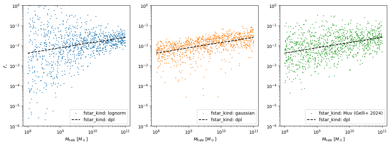
We model the stellar-to-halo ratio with a power-law function that depends on the hosting halo mass, such that:

\[f_\star(M_\mathrm{halo})= \frac{\Omega_\mathrm{m}}{\Omega_\mathrm{b}}\, \frac{2\cdot f_{\star,0}}{\left(\frac{M_\mathrm{halo}}{M_\mathrm{p}}\right)^{\gamma_1} + \left(\frac{M_\mathrm{halo}}{M_\mathrm{p}}\right)^{\gamma_2}} \left[1 + \left(\frac{M_\mathrm{t}}{M_\mathrm{halo}} \right)^{\gamma_3} \right]^{\gamma_4}\]

This double power-law model has seven free parameters and has beeing employed for study of the Cosmic Dawn, with \(\gamma_1 < 0\), \(\gamma_2 < 0\), \(\gamma_4 < 0\) and \(\gamma_3 > 0\). However, for reionization this can be simplified to a simple power-law for \(\gamma_1=\gamma_2\) and \(\gamma_3=\gamma_4=0\).

In the paremeter file, you can find these free parameters in the Sources group. To select this model you need to choose: fstar_kind: 'dpl'. Moreover, you have the seven free parameters: f0, Mt, Mp, g1, g2, g3 and g4.

Notice that one can select a mass independent model by setting \(\gamma_1=\gamma_2=\gamma_3=\gamma_4=0\).

# load source model
source_model = pc2r.source_model.StellarToHaloRelation(model=params['Sources']['fstar_kind'],
                                                       pars=params['Sources'],
                                                       cosmo=cosmo)

print('Model selected in the parameter file: %s' %params['Sources']['fstar_kind'])
print('Source variable in the parameter file:\n %s' %params['Sources'])

Model selected in the parameter file: dpl
Source variable in the parameter file:
 {'fstar_kind': 'dpl', 'fgamma_hm': 30, 'fgamma_lm': 0.0, 'Nion': 2000.0, 'f0': 0.1, 'Mt': '1e8', 'Mp': '1e10', 'g1': -0.3, 'g2': -0.3, 'g3': 0, 'g4': -0.0, 'fesc_model': 'power', 'f0_esc': 0.02, 'Mp_esc': '1e10', 'al_esc': -0.25, 'accretion_model': 'EXP', 'alpha_h': 0.79, 'bursty_sfr': 'no', 'beta1': 0.1, 'beta2': 1.5, 'tB0': 200.0, 'tQ_frac': 1.6, 'z0': 30.0, 't_rnd': 0}

# load source model
fstar_pars = {'Nion': 4., 'f0': 0.1, 'Mt': 1e8, 'Mp': 1e10, 'g1': -0.3, 'g2': -0.2, 'g3': 0.1, 'g4': -0.2, 'alpha_h': 0.79}
source_model = pc2r.source_model.StellarToHaloRelation(model='dpl', pars=fstar_pars, cosmo=cosmo)

fstar1 = source_model.deterministic(Mhalo=mhalo)
fstar2 = source_model.stochastic_lognormal(Mhalo=mhalo)
fstar3 = source_model.stochastic_Gaussian(Mhalo=mhalo, sigma=[1.]*mhalo.size)
fstar4 = source_model.fstar_from_Muv(Mhalo=mhalo, z=7.305)

fig, axs = plt.subplots(figsize=(15,5), ncols=3, nrows=1)
axs[0].scatter(mhalo, fstar2, s=1, color='tab:blue', label='fstar_kind: lognorm')
axs[1].scatter(mhalo, fstar3, s=1, color='tab:orange', label='fstar_kind: gaussian')
axs[2].scatter(mhalo, fstar4, s=1, color='tab:green', label='fstar_kind: Muv (Gelli+ 2024)')

for ax in axs:
    ax.loglog(mhalo, fstar1, color='black', ls='--', label='fstar_kind: dpl')
    ax.set_ylim(1e-6, 1)
    ax.set_xlabel(r'$M_\mathrm{halo}$ [$M_\odot$]')
    ax.legend(loc=4)

axs[0].set_ylabel(r'$f_\star$')
plt.show(), plt.clf()

(None, None)

<Figure size 640x480 with 0 Axes>

Escaping Fraction Model

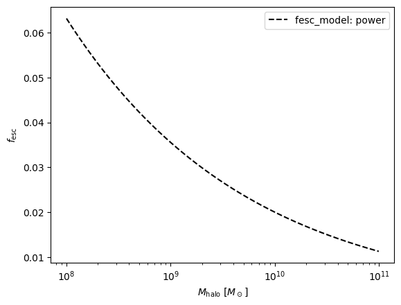
We model the stellar-to-halo ratio with a power-law function that depends on the hosting halo mass, such that:

\[f_\mathrm{esc}(M_\mathrm{halo})= f_\mathrm{esc,0}\, \left(\frac{M_\mathrm{halo}}{M_\mathrm{p,esc}} \right)^{\alpha_\mathrm{esc}}\]

This power-law model has three free parameters, \(f_\mathrm{esc,0}\), \(M_\mathrm{p,esc}\) and \(\alpha_\mathrm{esc} > 0\).

In the paremeter file, you can find these free parameters in the Sources group. To select this model you need to choose: fesc_model: 'power'. Moreover, you have the free parameters: f0_esc, Mp_esc and al_esc.

Notice that one can select a mass independent model by setting \(\alpha_\mathrm{esc}=0\).

fesc_pars = {'f0_esc': 0.02, 'Mp_esc': 1e10, 'al_esc': -0.25}
fesc_model = pc2r.source_model.EscapeFraction(model='power', pars=fesc_pars)

fesc1 = fesc_model.deterministic(Mhalo=mhalo)
plt.semilogx(mhalo, fesc1, color='black', ls='--', label='fesc_model: power')
plt.legend()
plt.xlabel(r'$M_\mathrm{halo}$ [$M_\odot$]'), plt.ylabel(r'$f_\mathrm{esc}$')
plt.show(), plt.clf()

(None, None)

<Figure size 640x480 with 0 Axes>

Halo Accretion Rate

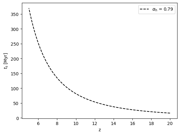
We model the halo accretion rate with a time scale variable, \(t_\mathrm{s}\), representing the source lifetime in our model.

\[\dot{M}_\mathrm{h}(z) = \frac{M_\mathrm{halo}(z)}{t_\mathrm{s}} = \frac{M_\mathrm{halo}(z)}{\left[ \alpha_\mathrm{h}(1+z)\,H(z) \right]^{-1}}\]

where \(\alpha_\mathrm{h}\) is a free parameter and \(H(z)\) is the Friedmann equation.

This analytical model assumes that the halos grow exponentially with the follwing relation:

\[M_\mathrm{halo}(z) = M_\mathrm{halo,0}\,e^{-\alpha_\mathrm{h}(z-z_0)}\]

Where at \(z_0\) the halo has initial mass of \(M_\mathrm{halo,0}\).

In the paremeter file, you can find the free parameter in the Sources group. To select this model you need to choose: acretion_model: 'EXP'. Moreover, you have the free parameters: alpha_h.

# get some redshifts
redshifts = np.linspace(20, 5, 100)

# calculate the time scale variable
t_s = (source_model.source_liftime(z=redshifts) * u.s).to('Myr')

plt.plot(redshifts, t_s, 'k--', label=r'$\alpha_\mathrm{h}$ = %.2f' %source_model.alph_h)
plt.xlabel('z'), plt.ylabel(r'$t_\mathrm{s}$ [Myr]')
plt.legend()
plt.show(), plt.clf()

(None, None)

<Figure size 640x480 with 0 Axes>

Bursty Star Formation Model

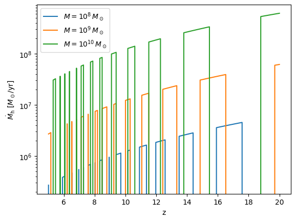
We have an analytical model for a bursty star-formation rate is defined with a bursty time-scale, \(t_\mathrm{B}\).

\[t_\mathrm{B}(M_h,t) = t_\mathrm{B,0}\cdot\left(\frac{M_h}{10^{10}\,M_\odot}\right)^{\beta_1}\cdot\left[H(t)(t-t_0)\right]^{\beta_2}\]

where \(t_\mathrm{B,0}\), \(\beta_1\), \(\beta_2\) and \(t_0\) are free parameters.

The length of the quiessence time is define by a factor parameters:

\[t_\mathrm{Q} = t_\mathrm{Q,frac} \cdot t_\mathrm{B}\]

In the paremeter file, you can find the free parameter in the Sources group. To select this model you need to choose: acretion_model: 'instant'. Moreover, you have the free parameters: beta1, beta2, tB0, z0 and tQ_frac.

bursty_pars = {'beta1': 0.1, 'beta2': 0.2, 'tB0': 300., 'tQ_frac': 0.95, 'z0': 30., 't_rnd': 0}
bursty = pc2r.source_model.BurstySFR(model='instant', pars=bursty_pars, alpha_h=0.79, cosmo=cosmo)

for m in [1e8, 1e9, 1e10]:
    # bursty SFR mask
    bh1 = bursty.instant_burst_or_quiescent_galaxies(mass=m, z=redshifts)

    # accreation rate (here in Myr)
    dotM = m/t_s.value

    plt.semilogy(redshifts, dotM*bh1, label=r'$M = 10^{%d}\,M_\odot$' %np.log10(m))

plt.ylabel(r'$\dot{M}_\mathrm{h}$ [$M_\odot/\mathrm{yr}$]'), plt.xlabel('z')
plt.legend()

<matplotlib.legend.Legend at 0x7d6705852cb0>

Sink Model

Here, below we show the sink models implemented in pyC\(^2\)Ray.

Clumping Factor

We define the gas clumping factor based on the cell-wise averaged quantities of the simulated intergalactic (IGM) density field:

\[\mathcal{C} = \frac{\left< n^2_\mathrm{IGM}\right>}{\left< n_\mathrm{IGM}\right>^2}\]

For homogeneous density, this quantity is close to unity, but if matter distribution within the volume can a few order of magnitude larger.

from IPython.display import Image, display
display(Image('example_clump.png'))

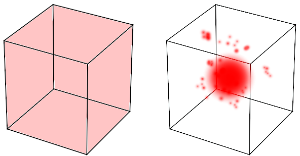
In the figure here above, we illustrate how a volume (a voxel in a simulation) can have the same density, \(\left<n_\mathrm{IGM}\right>\), but different clumping factor. In the left panel, an homogeneous field has \(\mathcal{C} = 1\), while for an highly inhomogeneous field (right panel) the clumping is, \(\mathcal{C} \geq 1\).

Here, we look at the clumping model implemented in pyC\(^2\)Ray that can be selected in the parameter file, parameters.yml, within the Sinks group and the variable clumping_model. Here, we refer the reader to Bianco et al. (2021) and Mao et al. (2019) for a review on the sub-grid clumping models illustrated here below.

The standard approach consider a constant clumping factor which is redshift, \(z\) and density-independent \(\delta_\mathrm{IGM}\). This can be selected in the parameter file by: clumping_model: 'constant' and is defined:

\[\mathcal{C}(z, \delta_\mathrm{IGM}) \equiv c^{ste}\]

The clumping value can be changed in the parameter file. The standard setup ignores the contribution by the sub-grid clumping inhomogeneity and set the value to one, clumping: 1.0.

params['Sinks']['clumping_model'] = 'constant'

print('Clumping model:', params['Sinks']['clumping_model'], 'with constant clumping factor:', params['Sinks']['clumping'])
sm = pc2r.sinks_model.SinksPhysics(params=params, N=params['Grid']['meshsize'])

const_clump = sm.calculate_clumping

# look at the min and max
print(const_clump.min(), const_clump.max(), const_clump.shape)

Clumping model: constant with constant clumping factor: 1.0
1.0 1.0 (256, 256, 256)

The bias homogeneous clumping (BHC) model considers a redshit evolving clumping factor that is independent of the sub-grid inhomogeneities. The model is defined as:

\[\mathcal{C}(z) = C_0\cdot e^{c_1\cdot z+c_2\cdot z^2} + 1\]

Here, the parameters \(C_0\), \(c_1\) and \(c_2\) are free parameters that have been fit to a high-resolution N-body simulation. These tables of fitting parameters can be found in pyC2R|ay/pyc2ray/tables/clumping/.

This can be selected in the parameter file by: clumping_model: 'redshift' in the Sinks group.

# modify the parameters file for a different clumping model
params['Sinks']['clumping_model'] = 'redshift'
print('Clumping model:', params['Sinks']['clumping_model'])

sm = pc2r.sinks_model.SinksPhysics(params=params, N=params['Grid']['meshsize'])

# select a redshift
z = 10.0
homogeneous_clump = sm.calculate_clumping(z=z)

# look at the min and max
print(homogeneous_clump.min(), homogeneous_clump.max(), homogeneous_clump.shape)

Clumping model: redshift
9.385467951445468 9.385467951445468 (256, 256, 256)

The ihomogeneous clumping (IC) model fit the clumping factor based on the simulated sub-grid density inhomogeneity. Therefore, the model read the density field an calculate the integalactic medium (IGM) overdensity, \(1+\delta_\mathrm{IGM}\). The model is then defined as:

\[\mathcal{C}(z, \delta_\mathrm{IGM}) = a\cdot (1+\delta_\mathrm{IGM})^2 + b \cdot (1+\delta_\mathrm{IGM}) + c\]

Here, the parameters \(a\), \(b\) and \(c\) are free parameters and the fitting parameters can be found in pyC2Ray/pyc2ray/tables/clumping/.

This can be selected in the parameter file by: clumping_model: 'density' in the Sinks group.

N = params['Grid']['meshsize']

# modify the parameters file for a different clumping model
params['Sinks']['clumping_model'] = 'density'
print('Clumping model:', params['Sinks']['clumping_model'])

sm = pc2r.sinks_model.SinksPhysics(params=params, N=N)

# select a redshift and create a mock density field
z = 10.0
overd = 1.0 + np.random.normal(loc=0, scale=0.1, size=(N, N, N))
ndens = cosmo.critical_density(z).cgs.value * overd

inhomogeneous_clump = sm.calculate_clumping(ndens=ndens, z=z)

# look at the min and max
print(inhomogeneous_clump.min(), inhomogeneous_clump.max(), inhomogeneous_clump.shape)

Clumping model: density
15.082506863292846 32.797772946000556 (256, 256, 256)

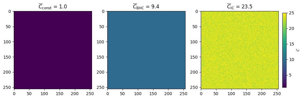
All the model return a 3D grid with the same mesh-size, and spatial resolution, of the density field. A series of tables, with the corresponding fitting parameters, can be found in pyC2Ray/pyc2ray/tables/clumping/.

To date, we have tables for different spatial resolution, i.e.: \(\Delta r = 2.094\), \(2.024\), \(1.518\), \(1.162\) and \(1.012\,\rm Mpc\) for a redshift range between \(z\in[45,\,7.3]\). In future work, we plan to increase the number of tables.

fig, axs = plt.subplots(figsize=(10, 8), nrows=1, ncols=3, constrained_layout=True)

axs[0].set_title('$\overline{C}_\mathrm{const}$ = %.1f' %const_clump.mean())
im = axs[0].imshow(const_clump[...,N//2], cmap='viridis', vmin=1, vmax=25)

axs[1].set_title('$\overline{C}_\mathrm{BHC}$ = %.1f' %homogeneous_clump.mean())
im = axs[1].imshow(homogeneous_clump[...,N//2], cmap='viridis', vmin=1, vmax=25)

axs[2].set_title('$\overline{C}_\mathrm{IC}$ = %.1f' %inhomogeneous_clump.mean())
im = axs[2].imshow(inhomogeneous_clump[...,N//2], cmap='viridis', vmin=1, vmax=25)
plt.colorbar(im, ax=axs[2], label=r'$\mathcal{C}$', pad=0.02, fraction=0.048)

<matplotlib.colorbar.Colorbar at 0x7d6705e82920>

# TODO: mean-free path