How to use the Chemistry Solver

In this tutorial, you can use the chemistry algorithm of pyC\(^2\)Ray as stand alone. However, this tutorial uses a simplified version of the full chemistry solver (doric method), without convergence loop for large time-step.

Therefore, we suggest the user to employ the chemistry solver as a stand alone only for very small time-step (\(\Delta t < 100\,\rm yr\)). Otherwise, convergence to the analytical solution is not granted.

Reionization Chemistry Equation for Hydrogen

Solving the hydrogen ionization fraction is not entirely trivial since this corresponds to a stiff partial differential equation. The evolution of ionized hydrogen can be written as:

\[\frac{dx_\mathrm{HII}}{dt} = (1-x_\mathrm{HII})\Gamma_\mathrm{HI} - x_\mathrm{HII}\, n_\mathrm{e} \alpha_\mathrm{HI}\]

The variables in this equation are:

• \(n_\mathrm{e}\) : the electron number density (itself depends on \(x_\mathrm{HII}\)).

• \(\alpha_\mathrm{HI}\) : the recombination coefficients for hydrogen (depends on the gas temperature). In our case, we assume the On-The-Spot (OTS) approximation, i.e. recombination to the ground state is locally absorbed). This approximation is equivalent to the Case B recombination coefficient.

• \(\Gamma_\mathrm{HI}\) : the photoionization rate for neutral hydrogen (itself depends on \(x_\mathrm{HI}\)).

We can find an analytical solution if we assume \(n_\mathrm{e}\), \(\alpha_\mathrm{HI}\) and \(\Gamma_\mathrm{HI}\) to be constant. For an inital condition \(x_\mathrm{HII,0}\), the solution is:

\[x_\mathrm{HII}(t) = x_\mathrm{eq}+\left(x_\mathrm{HII,0} + x_\mathrm{eq} \right)\,e^{t/t_\mathrm{i}}\]

With a time parameter:

\[t_\mathrm{i} = \frac{1}{\Gamma_\mathrm{HI} + n_\mathrm{e} \alpha_\mathrm{HI}}\]

The equilibrium solution:

\[x_\mathrm{eq} = \frac{\Gamma_\mathrm{HI}}{\Gamma_\mathrm{HI} + n_\mathrm{e} \alpha_\mathrm{HI}}\]

Using this solution and iterating for the electron density, we can derive an analytical solution for the time averaged chemistry solution (TACS) for a discrete time step \(\Delta t\) with solution:

\[\left< x_\mathrm{HII} \right> = \frac{1}{\Delta t} \int^{t+\Delta t}_{t} x_\mathrm{HII}(t')dt' = x_\mathrm{eq} + \left(x_\mathrm{HII,0} + x_\mathrm{eq} \right) \left(1 - e^{-\Delta t /t_\mathrm{i}} \right) \frac{t_\mathrm{i}}{\Delta t}\]

Below, we show a simple implementation of how to use the chemistry solver.

import numpy as np
import pyc2ray as pc2r
import matplotlib.pyplot as plt

import astropy.units as u
import astropy.constants as cst
from astropy.cosmology import Planck18 as cosmo

from tqdm import tqdm

In this example, we define some random density fields for the gas density ndens, temperature temp, ionization fraction xh, and photo-ionization rate phi_ion. These four fields can be a single value or a numpy array with the same shape.

mesh_shape = (10,10,10)

np.random.seed(2023)
# density field [g/cm^3]
ndens = np.random.normal(loc=1e-7, scale=1e-8, size=mesh_shape)

# temperature [K]
temp = np.ones(mesh_shape)*1e4

# Hydrogen ionization fraction
xh = np.random.uniform(low=0, high=0.1, size=mesh_shape)
xh_ini = xh

# photo-ionization rate [s^-1]
phi_ion = np.random.uniform(low=1e-13, high=1e-12, size=mesh_shape)

# clumping factor
clumping = np.ones(mesh_shape)

Run Time-Averaged Chemistry Solution

Define a time length dt (in seconds units) and loop over t_steps many time-steps.

The chemistry solver method employed in a pyC\(^2\)Ray assumes a constant electron density \(n_e\) and photo-ionization rate \(\Gamma_{\rm HI}\) within each time-step, \(\Delta t\) (which can be of several Myr). Moreover, the solution of the

Therefore, cosmological runs include a convergence loop to update the two fields and converge to the correct solution.

Therefore, if you wish to use the chemistry solver alone, you need to select a relatively small time length (\(\Delta t<100\, \rm yr\)), and this can depend on the strength of the source flux or ionization fraction of the voxel. For this reason, the code fails if more than 1% of the voxels do not converge.

# time-step
dt = 50*u.yr
t_steps = 1000

print('Volume-averaged ionized fraction at t=0: %.3f' %np.mean(xh_ini))

# array to show the time evolution of the solution
mean_xHII = np.zeros(t_steps)

# calculate ODE
for i in tqdm(range(t_steps)):
    new_xh = pc2r.hydrogen.hydrogenODE(dt=dt.cgs.value, ndens=ndens, temp=temp, xh=xh, phi_ion=phi_ion, clump=clumping)
    xh = new_xh

    # save value one voxel to show temporal evolution
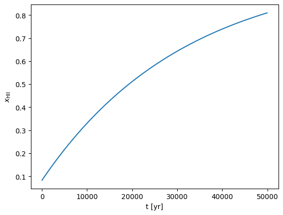
    mean_xHII[i] = xh[8,5,6]

print('Volume-averaged ionized fraction after t=%d %s: %.3f' %(dt.value*t_steps, dt.unit, np.mean(xh)))

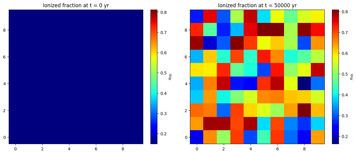
Volume-averaged ionized fraction at t=0: 0.050

100%|█████████████████████████████████████| 1000/1000 [00:00<00:00, 1061.30it/s]

Volume-averaged ionized fraction after t=50000 yr: 0.559

Plot the results the inital and final neutral fraction field.

fig, axs = plt.subplots(figsize=(12,5), ncols=2, nrows=1, layout="constrained")
axs[0].set_title('Ionized fraction at t = 0 %s' %dt.unit)
im = axs[0].imshow(xh_ini[:,mesh_shape[1]//2,:], origin='lower', cmap='jet', vmin=xh.min(), vmax=xh.max())
plt.colorbar(im, ax=axs[0], label=r'$x_{\rm HII}$')

axs[1].set_title('Ionized fraction at t = %d %s' %(dt.value*t_steps, dt.unit))
im = axs[1].imshow(xh[:,mesh_shape[1]//2,:], origin='lower', cmap='jet')
plt.colorbar(im, ax=axs[1], label=r'$x_{\rm HII}$')

<matplotlib.colorbar.Colorbar at 0x7688aa553940>

fig, axs = plt.subplots(figsize=(18,5), ncols=3, nrows=1)
axs[0].set_title('Density field')
im = axs[0].imshow(ndens[:,mesh_shape[1]//2,:], origin='lower', cmap='Purples')
plt.colorbar(im, ax=axs[0], label=r'$n_{\rm gas}$ [g/$\rm cm^{-3}$]')

axs[1].set_title('Photoionization rate')
im = axs[1].imshow(phi_ion[:,mesh_shape[1]//2,:], origin='lower', cmap='Oranges')
plt.colorbar(im, ax=axs[1], label=r'$\Phi_{\rm HI}$ [$\rm s^{-1}$]')

axs[2].set_title('Ionized fraction')
im = axs[2].imshow(xh[:,mesh_shape[1]//2,:], origin='lower', cmap='jet')
plt.colorbar(im, ax=axs[2], label=r'$x_{\rm HII}$')

<matplotlib.colorbar.Colorbar at 0x7688a9f836d0>

time_step = np.arange(0, t_steps)*dt
plt.plot(time_step, mean_xHII)
plt.xlabel('t [yr]'), plt.ylabel(r'$x_\mathrm{HII}$')
plt.show(), plt.clf()

(None, None)

<Figure size 640x480 with 0 Axes>